Penalised regression with multiple sets of prior effects

Implements penalised regression with multiple sets of prior effects

Usage

transreg(
  y,
  X,
  prior,
  family = "gaussian",
  alpha = 1,
  foldid = NULL,
  nfolds = 10,
  scale = "iso",
  stack = "sim",
  sign = FALSE,
  switch = FALSE,
  select = TRUE,
  track = FALSE,
  parallel = FALSE
)

Arguments

y: target: vector of length \(n\) (see family)
X: features: matrix with \(n\) rows (samples) and \(p\) columns (features)
prior: prior coefficients: matrix with \(p\) rows (features) and \(k\) columns (sources of co-data)
family: character "gaussian" (\(y\): real numbers), "binomial" (\(y\): 0s and 1s), or "poisson" (\(y\): non-negative integers);
alpha: elastic net mixing parameter (0=ridge, 1=lasso): number between 0 and 1
foldid: fold identifiers: vector of length \(n\) with entries from 1 to nfolds
nfolds: number of folds: positive integer
scale: character "exp" for exponential calibration or "iso" for isotonic calibration
stack: character "sta" (standard stacking) or "sim" (simultaneous stacking)
sign: sign discovery procedure: logical (experimental argument)
switch: choose between positive and negative weights for each source: logical
select: select from sources: logical
track: show intermediate output (messages and plots): logical
parallel: logical (see cv.glmnet)

Value

Returns an object of class transreg. Rather than accessing its slots (see list below), it is recommended to use methods like coef.transreg() and predict.transreg().

slot base: Object of class glmnet. Regression of outcome on features (without prior effects), with \(1 + p\) estimated coefficients (intercept + features).
slot meta.sta: NULL or object of class glmnet. Regression of outcome on cross-validated linear predictors from prior effects and estimated effects, with \(1 + k + 2\) estimated coefficients (intercept + sources of co-data + lambda_min and lambda_1se).
slot meta.sim: NULL or object of class glmnet. Regression of outcome on meta-features (cross-validated linear predictors from prior effects) and original features, with \(1 + k + p\) estimated coefficients (intercept + sources of co-data + features).
slot prior.calib: Calibrated prior effects. Matrix with \(p\) rows and \(k\) columns.
slot data: Original data. List with slots y, X and prior (see arguments).
slot info: Information on call. Data frame with entries \(n\), \(p\), \(k\), family, alpha, scale and stack (see details and arguments).

Details

\(n\): sample size
\(p\): number of features
\(k\): number of sources

References

Armin Rauschenberger, Zied Landoulsi, Mark A. van de Wiel, and Enrico Glaab (2023). "Penalised regression with multiple sets of prior effects". Bioinformatics (In press). doi:10.1093/bioinformatics/btad680 armin.rauschenberger@uni.lu

Examples

#--- simulation ---
n <- 100; p <- 500
X <- matrix(rnorm(n=n*p),nrow=n,ncol=p)
beta <- rnorm(p)*rbinom(n=p,size=1,prob=0.2)
prior1 <- beta + rnorm(p)
prior2 <- beta + rnorm(p)
y_lin <- X %*% beta
y_log <- 1*(y_lin > 0)

#--- single vs multiple priors ---
one <- transreg(y=y_lin,X=X,prior=prior1)
two <- transreg(y=y_lin,X=X,prior=cbind(prior1,prior2))
weights(one)
#> [1] 0.6724394
weights(two)
#> [1] 0.6208604 0.5642326

# \donttest{
#--- linear vs logistic regression ---
lin <- transreg(y=y_lin,X=X,prior=prior1,family="gaussian")
log <- transreg(y=y_log,X=X,prior=prior1,family="binomial")
hist(predict(lin,newx=X)) # predicted values

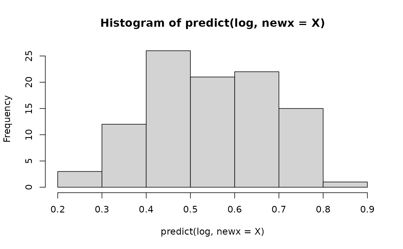
hist(predict(log,newx=X)) # predicted probabilities


#--- ridge vs lasso penalisation ---
ridge <- transreg(y=y_lin,X=X,prior=prior1,alpha=0)
lasso <- transreg(y=y_lin,X=X,prior=prior1,alpha=1)
# initial coefficients (without prior)
plot(x=coef(ridge$base)[-1]) # dense

plot(x=coef(lasso$base)[-1]) # sparse

# final coefficients (with prior)
plot(x=coef(ridge)$beta) # dense

plot(x=coef(lasso)$beta) # not sparse


#--- exponential vs isotonic calibration ---
exp <- transreg(y=y_lin,X=X,prior=prior1,scale="exp")
iso <- transreg(y=y_lin,X=X,prior=prior1,scale="iso")
plot(x=prior1,y=exp$prior.calib)

plot(x=prior1,y=iso$prior.calib)


#--- standard vs simultaneous stacking ---
prior <- c(prior1[1:250],rep(0,250))
sta <- transreg(y=y_lin,X=X,prior=prior,stack="sta")
sim <- transreg(y=y_lin,X=X,prior=prior,stack="sim")
plot(x=coef(sta$base)[-1],y=coef(sta)$beta)

plot(x=coef(sim$base)[-1],y=coef(sim)$beta)# }