Plot transreg-object

Plot transreg-object

Usage

# S3 method for transreg
plot(x, stack = NULL, ...)

Arguments

x

object of type transreg

stack

character "sta" (standard stacking) or "sim" (simultaneous stacking)

...

(not applicable)

Value

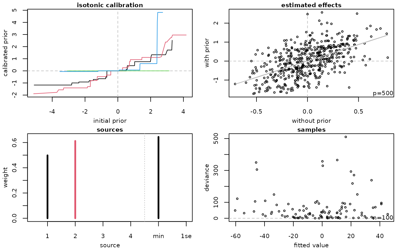
Returns four plots.

• top-left: Calibrated prior effects (\(y\)-axis) against original prior effects (\(x\)-axis). Each line is for one source of prior effects, with the colour given by grDevices::palette() (black: 1, red: 2, green: 3, blue: 4, ...).

• top-right: Estimated coefficients with transfer learning (\(y\)-axis) against estimated coefficients without transfer learning (\(x\)-axis). Each point represents one feature.

• bottom-left: Estimated weights for sources of prior effects (labels 1 to \(k\)), and either estimated weights for lambda.min and lambda.1se models (standard stacking) or estimated weights for features (simultaneous stacking).

• bottom-right: Absolute deviance residuals (\(y\)-axis) against fitted values (\(x\)-axis). Each point represents one sample.

References

Armin Rauschenberger, Zied Landoulsi, Mark A. van de Wiel, and Enrico Glaab (2023). "Penalised regression with multiple sets of prior effects". Bioinformatics (In press). doi:10.1093/bioinformatics/btad680 armin.rauschenberger@uni.lu

See also

Methods for objects of class transreg include coef and predict.

Examples

#--- simulation ---
set.seed(1)
n <- 100; p <- 500
X <- matrix(rnorm(n=n*p),nrow=n,ncol=p)
beta <- rnorm(p) #*rbinom(n=n,size=1,prob=0.2)
prior1 <- beta + rnorm(p)
prior2 <- beta + rnorm(p)
prior3 <- rnorm(p)
prior4 <- rnorm(p)
y <- X %*% beta

prior <- cbind(prior1,prior2,prior3,prior4)
object <- transreg(y=y,X=X,prior=prior,alpha=0,stack=c("sta","sim"))

plot(object,stack="sta")